
Neural Networks For Feature Analysis
Introductions
Mayank Barad
Rising Senior pursuing BSE in Computer Engineering and Computer Science
Daksh Khetarpaul
Rising Junior pursuing BSE in Computer Engineering
Katherine Lew
Rising Sophomore pursuing BS in Finance and Computer Science
Advisors - Dr. Richard Howard, Dr. Richard Martin
Project Poster

Project Description
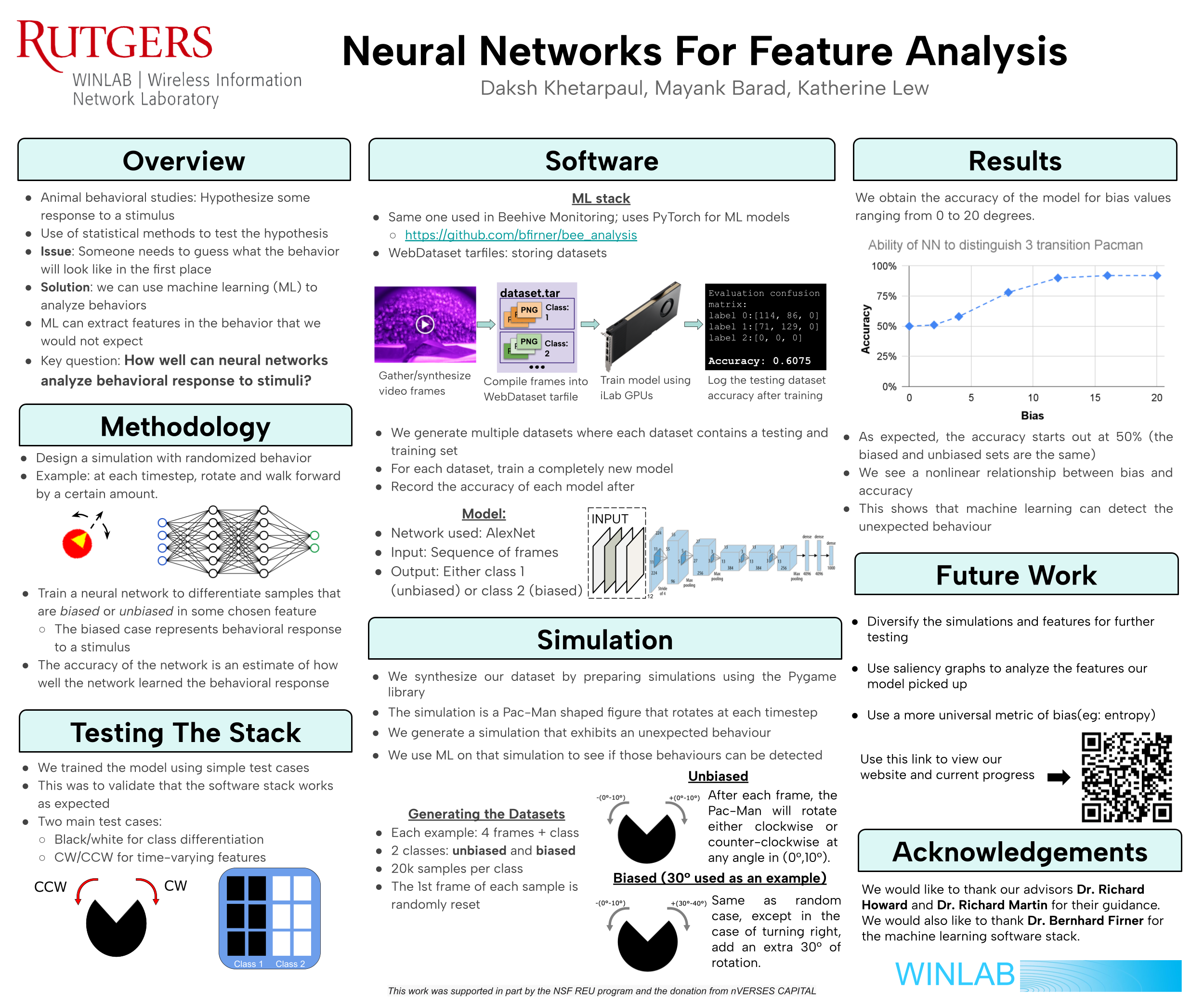
Neural networks have a long history of being used for classification, and more recently content generation, Example classifiers including, image classification between dogs and cats, text sentiment classification. Example generative networks include those for human faces, images, and text. Rather than classification or generation, this work explores using networks for feature analysis. Intuitively, features are the high level patterns that distinguish data, such as text and images, into different classes. Our goal is to explore bee motion datasets to qualitatively measure the ease or difficulty of reverse-engineering the features found by the neural networks.
Week 1 Progress
- Defining objectives: We defined the objective of our project: to explore how well behavioral anomalies and patterns in bees are recognized by a neural network.
Neural Networks for Feature Analysis and Hive Monitoring are interrelated. The Hive Monitoring project is based on the hypothesis that changes in the earth's magnetic fields due to radio waves are affecting bee behavior. Their goal is to determine if bees exposed to a magnetic field behave differently than un-exposed bees. Our goal is to explore the use of Neural Networks to detect these changes.
How effective are neural networks at detecting minute changes in bee behavior?
- Set up software: We set up Github and iLab accounts to collaborate and run the machine learning behavioral detection code, respectively.
- Research neural networks: We researched neural networks to become familiar with the model. Looked into concepts like , , and .
Week 2 Progress
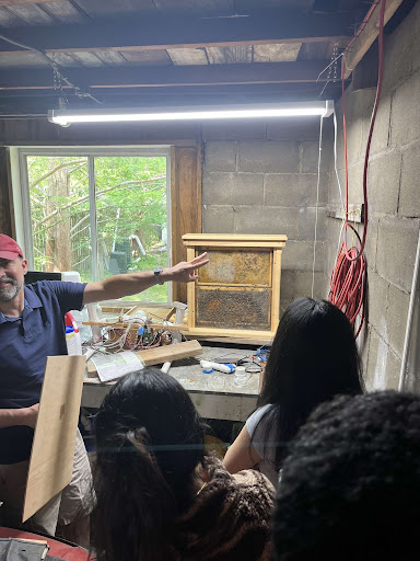
- Observation: Visited the beehive to observe the behavior of real bees
- Simulation: Made a prototype simulator with pygame - Rejected(pretty obvious reasons)
- Power Law: Integrated "Power Law" for a more natural bee motion
 First Prototype →
  Applying "Power Law" →
Week 3 Progress
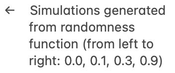
- Randomness Function:We programmed a function that allows the user to adjust the degree of randomness of synthetic bee motion along a spectrum. 0.0 represents the "bee" moving in a completely random motion, and 1.0 represents the "bee" moving via a distinct non-random pattern like a clockwise circle.
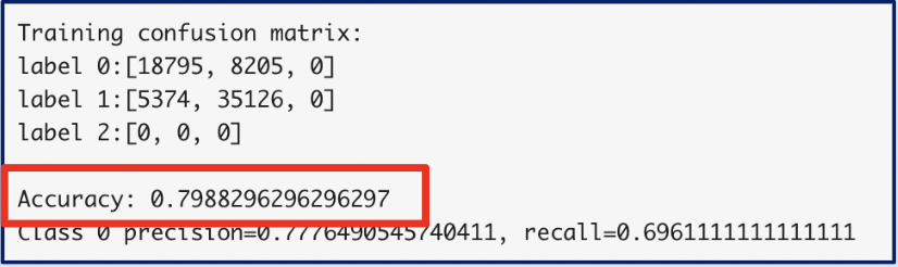
- Train model: We used the randomness function to trained the machine learning model (AlexNet adjacent) to try to detect the difference between the random and non-random behavioral patterns. The model outputted a confusion matrix and an accuracy of 0.798 in identifying randomness.
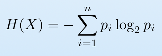
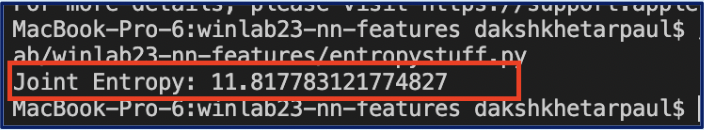
- Shannon's Entropy: We researched Shannon's Entropy Function as a measure of the model's accuracy and created a program that automates the calculation of the joint entropy of two discrete random variables within the random system (e.g angle and distance)


Weeks 4 and 5 Progress
- Validate results: We discovered that there was a mistake in our training data, so last week's training results were null. There was a bias in the input data, and irrelevant learning happened.
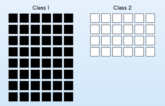
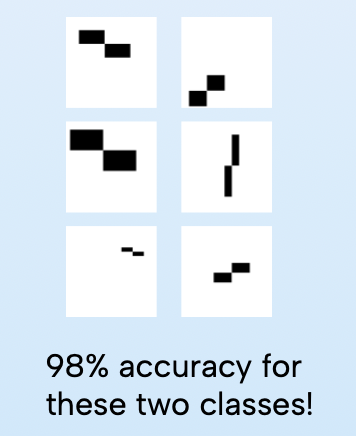
- Retrain model: We retrained the machine learning model using simpler test cases, like the black-white frame test. With simple black-and-white classes, our model obtained 100% accuracy. With more complicated classes, our model obtained 98% accuracy.
- Reformat tar files: We altered the program to reformat the training data. Instead of combining the frames of the random bee simulator into a video format, we compiled the data into a tar file, which consists of a png, a class, and a metadata file for each frame in the simulation. We will use these tar files as training data for the model.
Week 6 Progress
- Time Varying Features: In order to train the model to capture time-varying features (motion), we increased the channels while keeping the same kernel size. This works for small movements in the training data.
- Clockwise-Anticlockwise Test: With the time-varying features accounted for, we began to train the model with patterns of motion instead of simple black-and-white frames. For instance, we created training data with one class of frames that move in a clockwise direction and one class of frames that move in a counterclockwise direction. Can the model detect left versus right rotations?
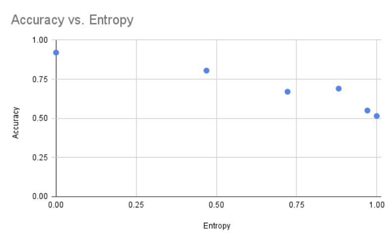
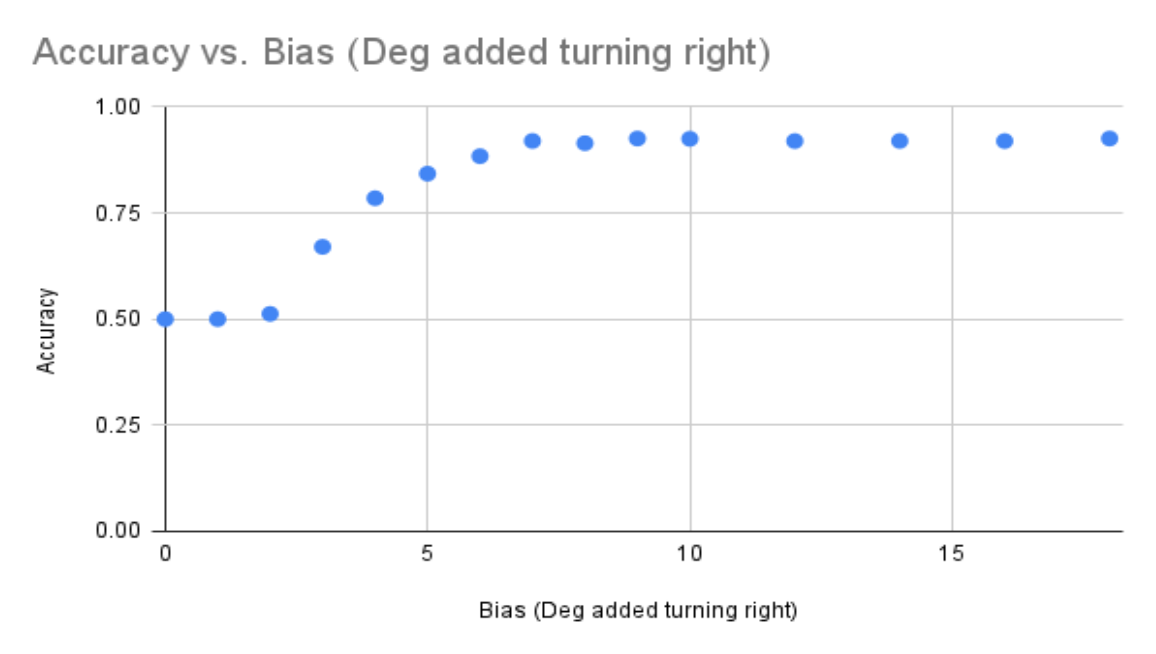
- Entropy v. Accuracy Graphs: We created a graph from our model output data to derive the relation between entropy versus accuracy.


Week 7 Progress
- Testing complicated patterns: We tested training data with more complicated patterns of movement. For instance, we trained the model with one class of frames moving in a completely random pattern and the other moving with a 3-degree bias to the right. After running 10,000 samples, we obtained 50% accuracy. We hypothesize 3 potential causes of the low accuracy: 1) sample size was too small 2) there was a problem in our datasets 3) there was an error in executing the software stack
- Testing with new bias: To rectify the issue, we changed the bias from 3 degrees to 30 degrees. The model was able to identify the change in bias with a 93% accuracy on 10,000 samples.


Week 8/9 Progress
- Slurm: Each training run of a dataset takes about 2-3 hours and generates one point (one accuracy and one bias) on the accuracy v. bias graph. Since many points are necessary to identify a consistent pattern between accuracy and bias, the graph could take days to create. We decided to use Sclurm workload manager to submit multiple jobs to iLab that run in parallel saving massive amounts of time.
- Automation of model training: We wrote a script that generates several datasets, trains the model using each of those datasets (with Sclurm), and outputs a final graph plotting accuracy v. bias (one point on the graph for each dataset). Since the generation and training process takes hours, this script saves the time required in manually running the model for each dataset.
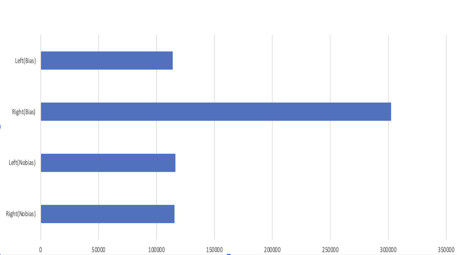
- Testing the simulator: We tested the model with a low bias (8 degrees) and obtained an abnormally low accuracy of 50%. To fix this issue, we decided to look back at the code and test the simulator itself to see if it is rotating or not rotating in the way we intended. We wrote a program with a count variable to keep track of the number of left versus right turns in each dataset and display a bar graph with these counts. For instance, in the "no bias" dataset the left and right bars are even because there is no bias, and the number of left turns equals the number of right turns. In the "bias" dataset, the bar for the right turns is significantly higher than that of the left turns, revealing a bias in the dataset that causes the bee to turn to the right. This graph confirms the legitimacy of our simulator (creating one biased and one non-biased dataset).


Attachments (30)
-
unnamed.jpg
(65.5 KB
) - added by 3 years ago.
bee garage
- jitterbug.mov (155.9 KB ) - added by 3 years ago.
- powerbee.mov (245.4 KB ) - added by 3 years ago.
- powerbee2.mov (194.8 KB ) - added by 3 years ago.
- 0.0.mov (275.2 KB ) - added by 3 years ago.
-
0.1.mov
(275.5 KB
) - added by 3 years ago.
Bee simulator set at 0.1 randomness
-
0.3.mov
(294.6 KB
) - added by 3 years ago.
Simulator set at 0.3 randomness
-
0.9.mov
(291.0 KB
) - added by 3 years ago.
Simulator set at 0.9 randomness
- Screen Shot 2023-07-13 at 2.16.03 PM.png (40.1 KB ) - added by 3 years ago.
-
Screen Shot 2023-07-13 at 2.16.03 PM.2.png
(40.1 KB
) - added by 3 years ago.
Shannon's entropy function
- Screen Shot 2023-07-19 at 10.44.07 AM.png (286.4 KB ) - added by 3 years ago.
- Screen Shot 2023-07-19 at 10.46.33 AM.png (104.1 KB ) - added by 3 years ago.
- Screen Shot 2023-07-19 at 11.40.37 AM.png (19.7 KB ) - added by 3 years ago.
- Screen Shot 2023-07-19 at 11.36.05 AM.png (114.0 KB ) - added by 3 years ago.
- Screen Shot 2023-07-19 at 11.38.38 AM.png (58.9 KB ) - added by 3 years ago.
- Screen Shot 2023-07-19 at 12.23.26 PM.png (42.0 KB ) - added by 3 years ago.
- anticlockwise.gif (2.4 MB ) - added by 3 years ago.
- clockwise.gif (2.7 MB ) - added by 3 years ago.
- yesbias_AdobeExpress.gif (1.1 MB ) - added by 3 years ago.
- nobias_AdobeExpress.gif (818.2 KB ) - added by 3 years ago.
- Screen Shot 2023-08-07 at 3.11.34 PM.png (95.6 KB ) - added by 3 years ago.
- Screen Shot 2023-08-07 at 3.22.19 PM.png (83.0 KB ) - added by 3 years ago.
- 0.0.gif (239.9 KB ) - added by 3 years ago.
- 0.3.gif (146.5 KB ) - added by 3 years ago.
- 0.4.gif (152.2 KB ) - added by 3 years ago.
- 0.9.gif (148.0 KB ) - added by 3 years ago.
- jitterbug2.gif (413.3 KB ) - added by 3 years ago.
- 0.1.gif (152.2 KB ) - added by 3 years ago.
- NN_poster.pptx.png (1004.9 KB ) - added by 3 years ago.
- NN_poster.pptx.pdf (607.2 KB ) - added by 3 years ago.