
| Version 83 (modified by , 2 years ago) ( diff ) |
|---|
Signal Avoidance Using 5G
WINLAB Summer Internship 2024
Advisors: Dr. Predrag Spasojevic
Group Members: Wesley Chen
Overview
Problem:
In recent years, there has been a desire to expand the bandwidth of communication standards such as LTE and 5G. However, at many of the bandwidths that are desired to be used, there exist legacy signals that cannot be interfered with. This is made even more difficult by Adjacent Channel Interference (ACI), when signals with very close, but distinct frequencies still impede each other.
Goal:
Build the framework to test signal avoidance.
Devices
Rhode & Schwarz SMW200A
The Rhode & Schwarz SMW200A is a vector signal generator with the ability to output signals from 100kHz to 40GHz with a 50 ohm impedance. The SMW200A has the ability to modulate a carrier signal with an arbitrary waveform (.wv file). For the extent of this project, this waveform was generated in python on a personal computer and uploaded to the machine via the ftp protocol.
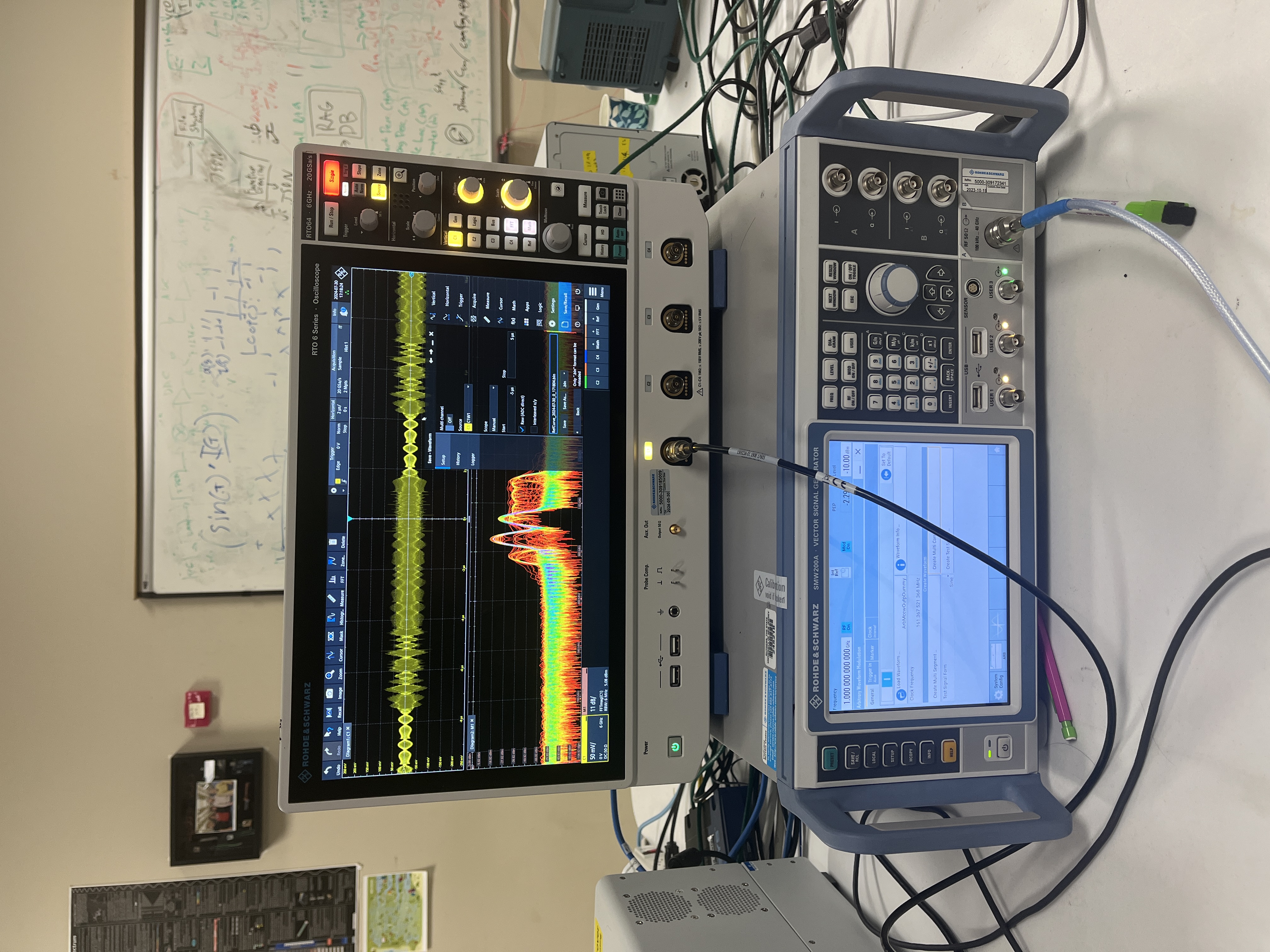
Rhode & Schwarz RTO 6 series
The Rhode & Schwarz RTO 6 series is an oscilloscope with the ability to read signals up to 6GHz and a sample rate of 20 giga-samples per second, although when downloading files from the machine, they are unconverted to 100 giga-samples per second. The RTO has built in mathematical functions such as FFTs to display the frequency domain on the machine. Additionally, as hinted earlier, the RTO can save waveforms in a .csv file which can be downloaded through network (the RTO operates as a windows machine). This file can be analyzed on a personal computer.

Top: RTO 6 series, Bottom: SMW200A
Concepts
What is a Signal?
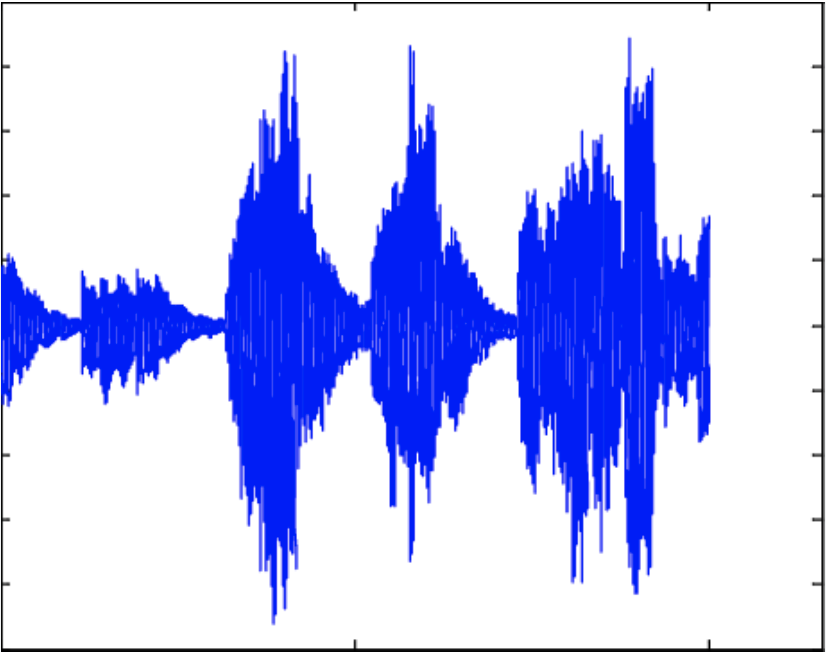
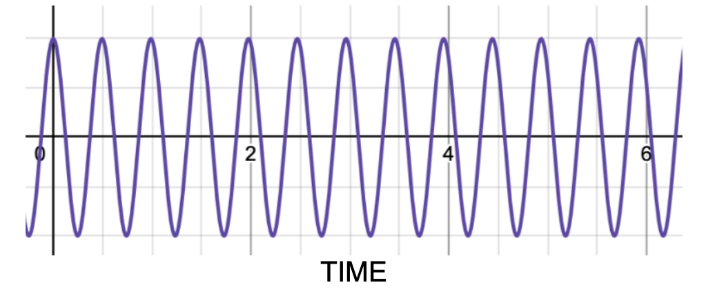
Undoubtedly, you have seen audio signals like the one shown below. In fact, Audio and Radio have many links to each other and the audio signal below could very well have been a radio signal.

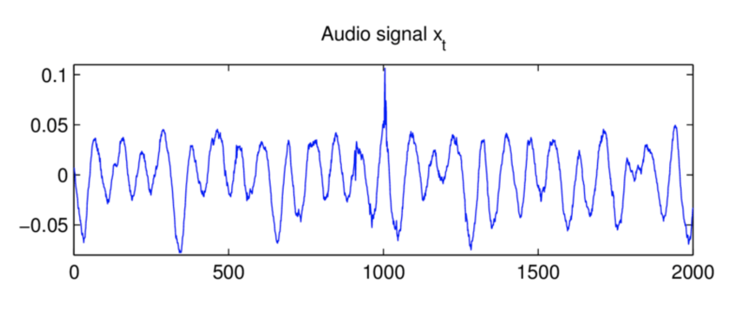
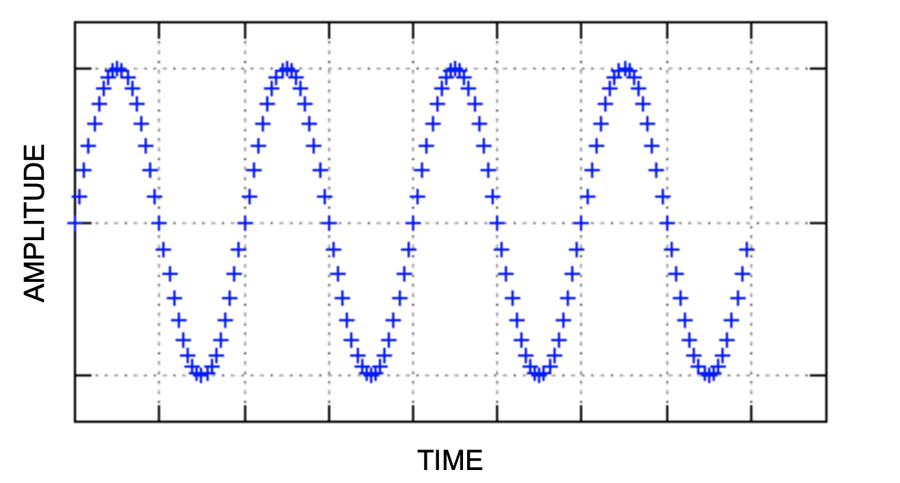
If you would have zoomed into that audio signal you would have seen something like the image below.

You may notice that this looks strikingly similar to some sort of sine wave and you would be 100% correct. Every signal can be thought of as a combination of sine waves. Each of theses sine waves has its own frequency and phase, meaning how fast it goes up and down and where the sine wave is centered, respectively.
Frequency Domain
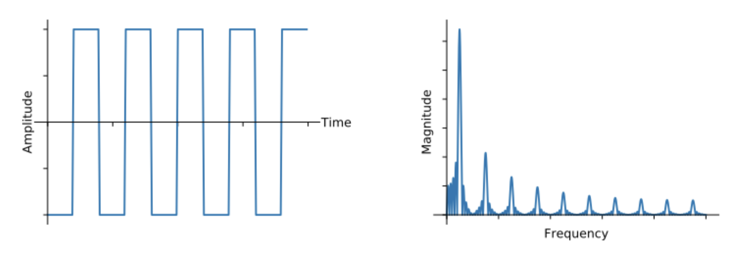
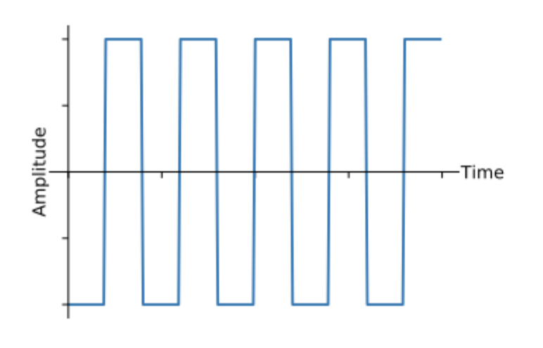
Because every signal is composed of sine waves of varying frequency and phase, we can actually represent the signals in terms of the frequencies and phases of those sine waves. This is called the Frequency Domain and is an equivalent representation for any signal. Below and left is a square wave in the time domain and to the right is the same signal in the frequency domain.

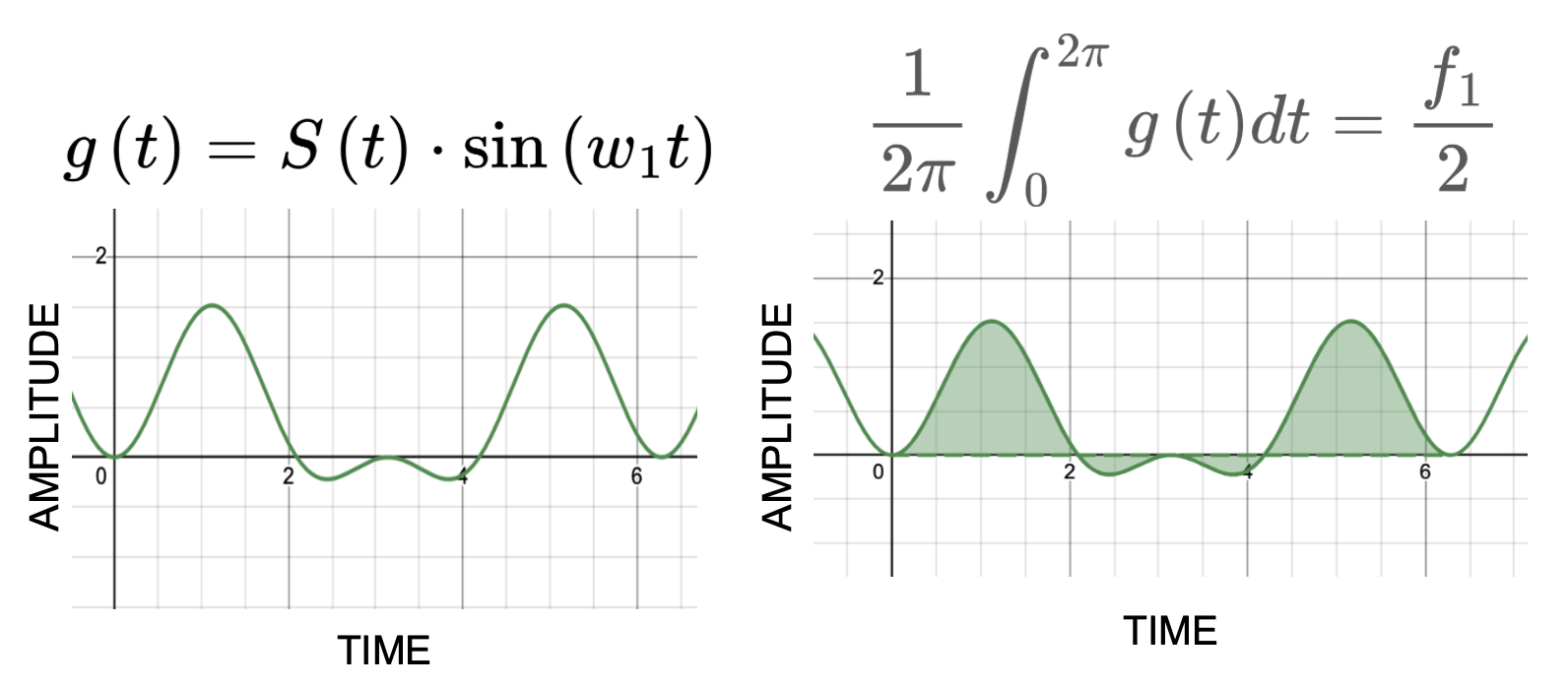
The conversion from time domain to the frequency domain occurs by multiplying each possible frequency sine wave with the signal and integrating over 1 period. This gives the magnitude of that frequency in the signal. In reality, an algorithm call Fast Fourier Transform (FFT) is used to do this multiplication and integration much quicker. FFT is a divide and conquer algorithm that makes use of complex number properties.

Complex Signals
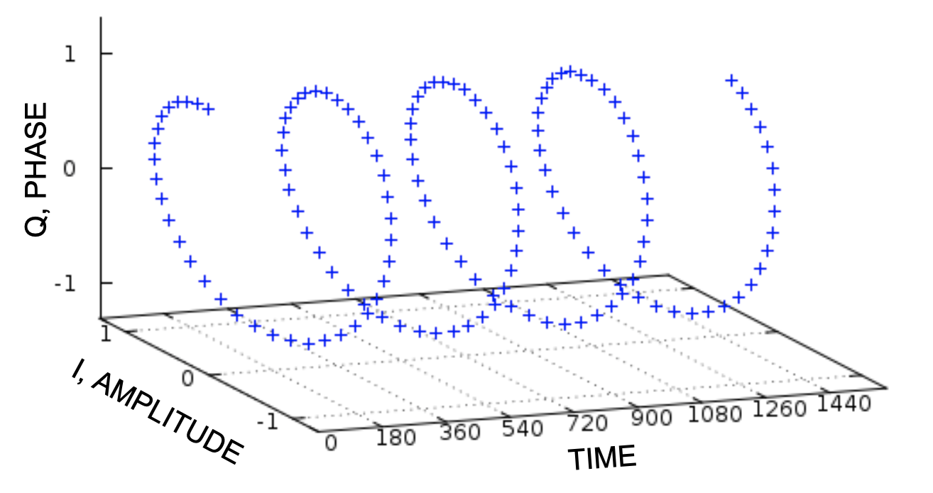
Speaking of complex number properties, signals can also be represented as complex numbers. While we may think of signals as up and down waves, shown left. In reality, signals can be complex 3 dimensional patterns, shown right.


The axis going into the page is the time and the vertical / horizontal axis are the phase and amplitude respectively. There are many other ways to think about these axis as well including the coefficients of sine and cosine waves and most notably real and imaginary numbers. This representation gives rise to a new way to represent the signal algebraically as well. S(t) = I(t) + Q(t)i, where S(t) is the signal, I(t) is the real component, Q(t) is the imaginary component and i is the imaginary number sqrt(-1). This imaginary number representation is advantageous in making the math in later stages much simpler.

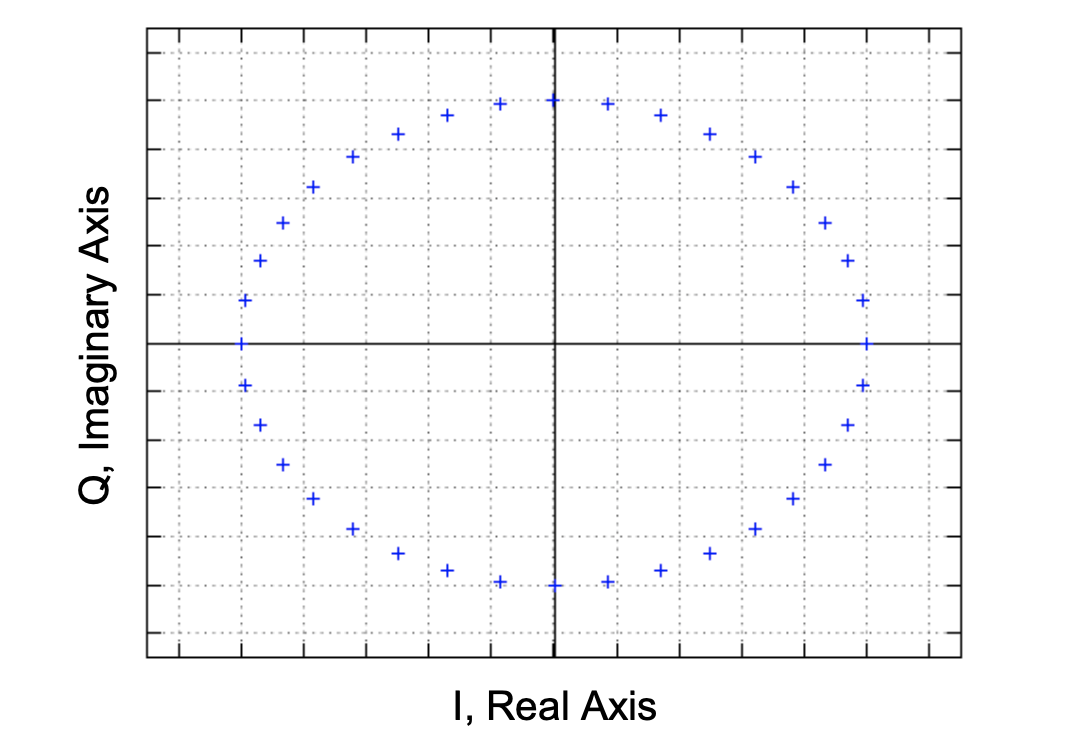
The complex signal representation also leads to something known as IQ plots, shown above. This is simply a plot of all points (I(t), Q(t)), placing I(t) on the horizontal/real axis and Q(t) on the vertical/imaginary axis. This graph can also be created by observing the 3 dimensional graph from the front face.
Modulation
In order to send signals as higher frequencies, we use a technique call modulation. We take the real part, I(t), of a signal and multiply it with a sine wave of the desired high frequency and the imaginary part, Q(t) with a cosine wave of that same frequency.
S(t) = I(t) + Q(t)i → I(t)*sin(wt) + Q(t)*cos(wt)
Note how the resulting signal is always real, even if the original signal had an imaginary component. It is important to remember that even though complex/imaginary signals are useful for various reasons, they don't actually exist in the real world because… well, they are imaginary!


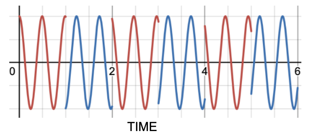
Example of a sine wave modulated by a square wave (right). The square wave (middle) switches between 1 and -1 causing the sine wave (left) the flip over and over again.
BPSK
What you see above is actually exactly what one signal technique known as BPSK is. BPSK stands for Binary Phase Shift Keying. It can only take on 2 different values every symbol, aka, one bit per symbol. Other methods such as QPSK and QAM can send multiple bits per symbol. It turns out that because of this 1 bit per symbol property, the IQ plot for any BPSK signal is always exactly 2 points. (1, 0) and (-1, 0). I(t) is either -1 or 1 and Q(t) is always 0. So, BPSK signals don't have imaginary components, not that that's relevant as we will be modulating anyways.

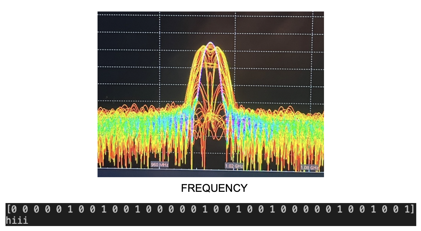
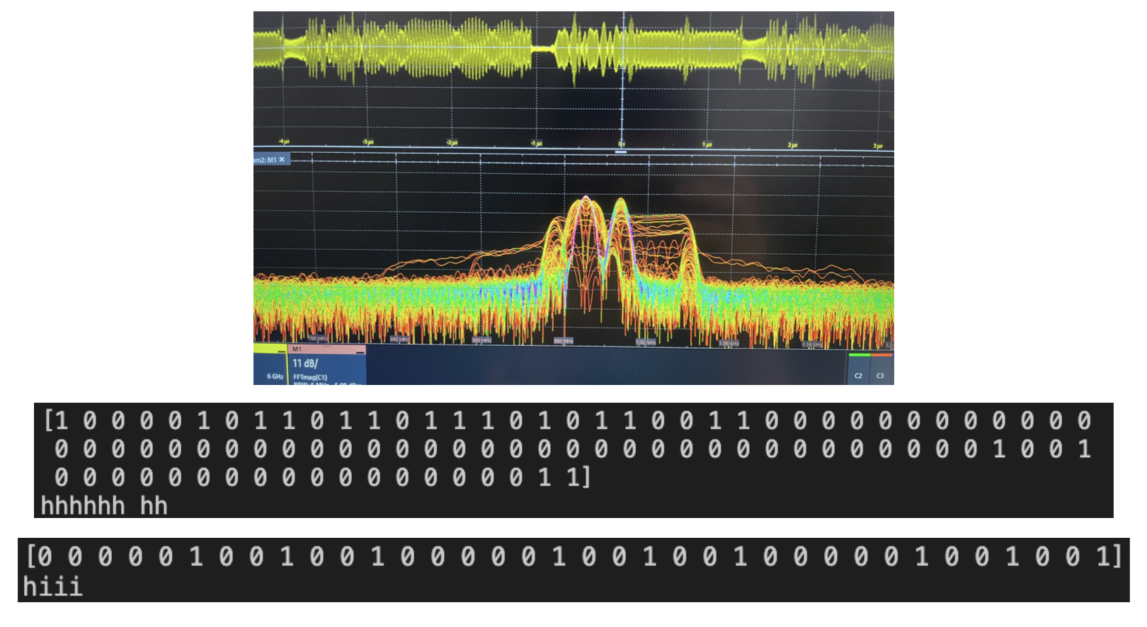
A BPSK signal has been received, on the top is frequency domain of the signal and on the bottom, the message "hiii".
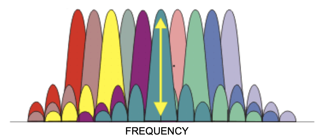
OFDM
OFDM is another signal technique, although this technique "sits" one layer above BPSK. The idea is to split up the bandwidth of a signal into multiple smaller bands and each of those carry data. OFDM stands for Orthogonal Frequency Division Multiplexing and the word "Orthogonal" indicates that the smaller bands do not interfere with each other. Note that the data rate on an OFDM and BPSK signal is the same as the smaller bands on OFDM lead to a slower rates on each channel.

Synchronization
In order to determine the bits from a signal we first have to get our IQ data from the signal. This is done by multiplying by sine and cosine waves of the carrier frequency.
S(t) = I(t) + Q(t)i
- S(t)*sin(wt) → low pass filter → I(t)
- S(t)*cos(wt) → low pass filter → Q(t)
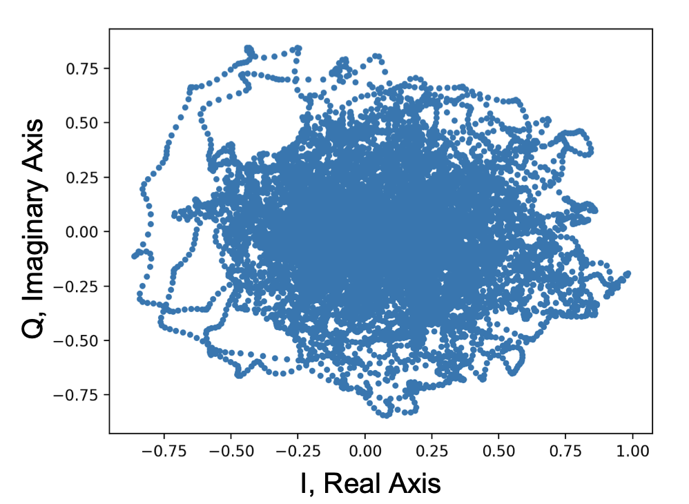
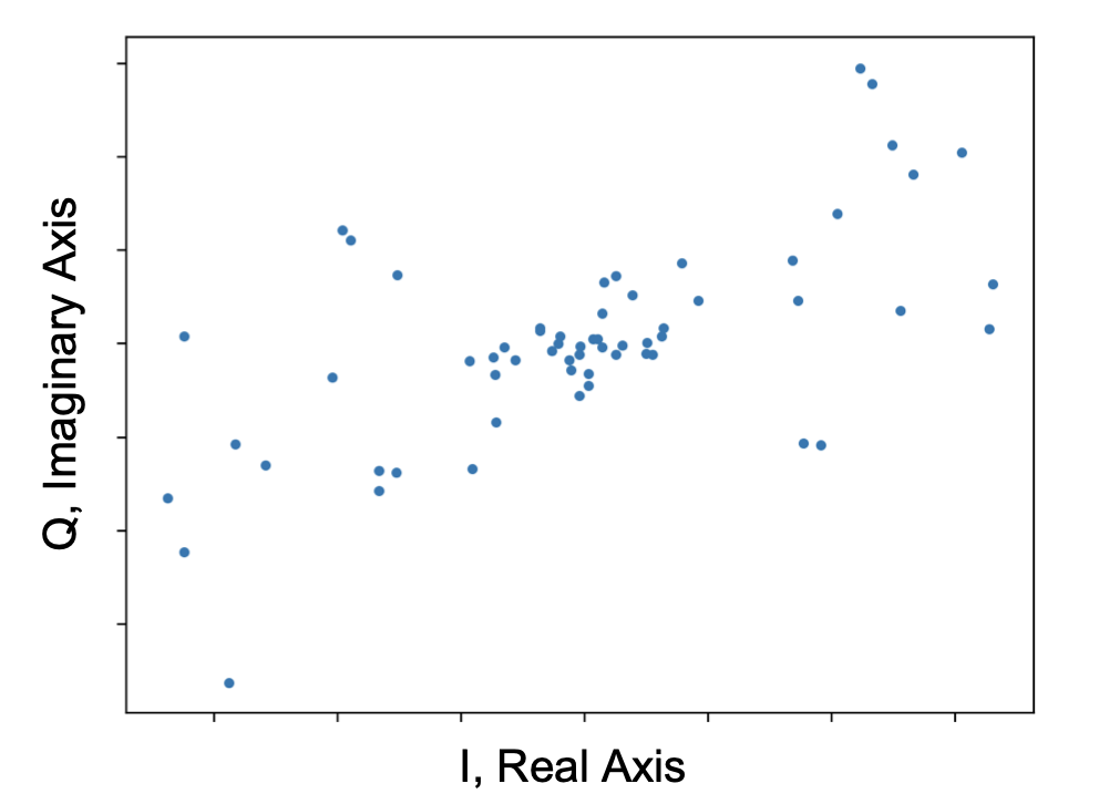
However, we don't know the phase of the sine wave. Another way to think about this is we don't know when to start receiving the signal. AND, even though the machine might tell us that the carrier is 1 GHz, there's no way it can send EXACTLY 1 GHz and might actually be something like 999.9 MHz. If we don't account for these, we get an IQ plot that looks like below. This signal is BPSK so we expect IQ to be across the real axis, though that's clearly not what we received.

The solution to this is to add something known as a barker code to the beginning of our signal. This is a special code that is "random," but both receiver and transmitter know what it is. So, at the transmitter, we compare the barker code to every timestamp in the signal and see which timestamps match the closest. We then know that the barker code occurred at those locations. Knowing one barker code can tell us where the signal starts. Knowing two can tell us the frequency offset based on the time difference between the two.

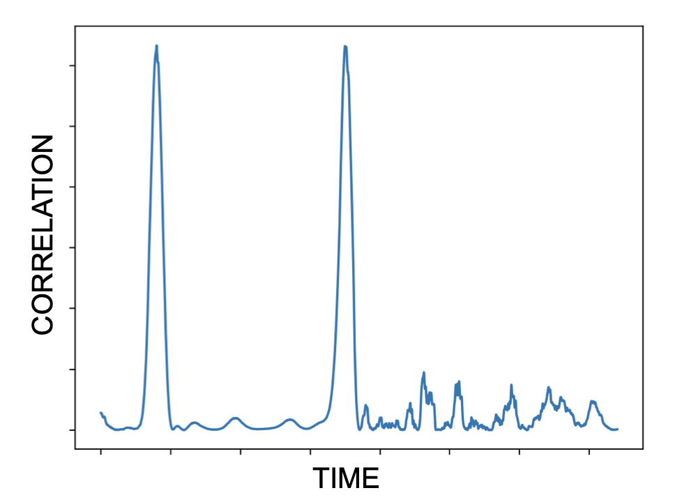
In reality this is done using a mathematical tool called correlation which compares multiplies the two signals at every time point (you can imagine the shorter barker code scrolling across the longer signal) and takes the integral/area under curve. After correlating with both I and Q, the result of each is squared and added together. The final correlation is shown below left.


After finding the frequency offset and phase, we can multiply each IQ sample by some exponential e(-i*<delta>) where <delta> stands in for the error / angle offset of that sample. When multiplying numbers in the complex plane, the angle of the two are added allowing us to easily correct every sample. Now we see why complex numbers are useful. The corrected IQ samples are shown above right.
Results
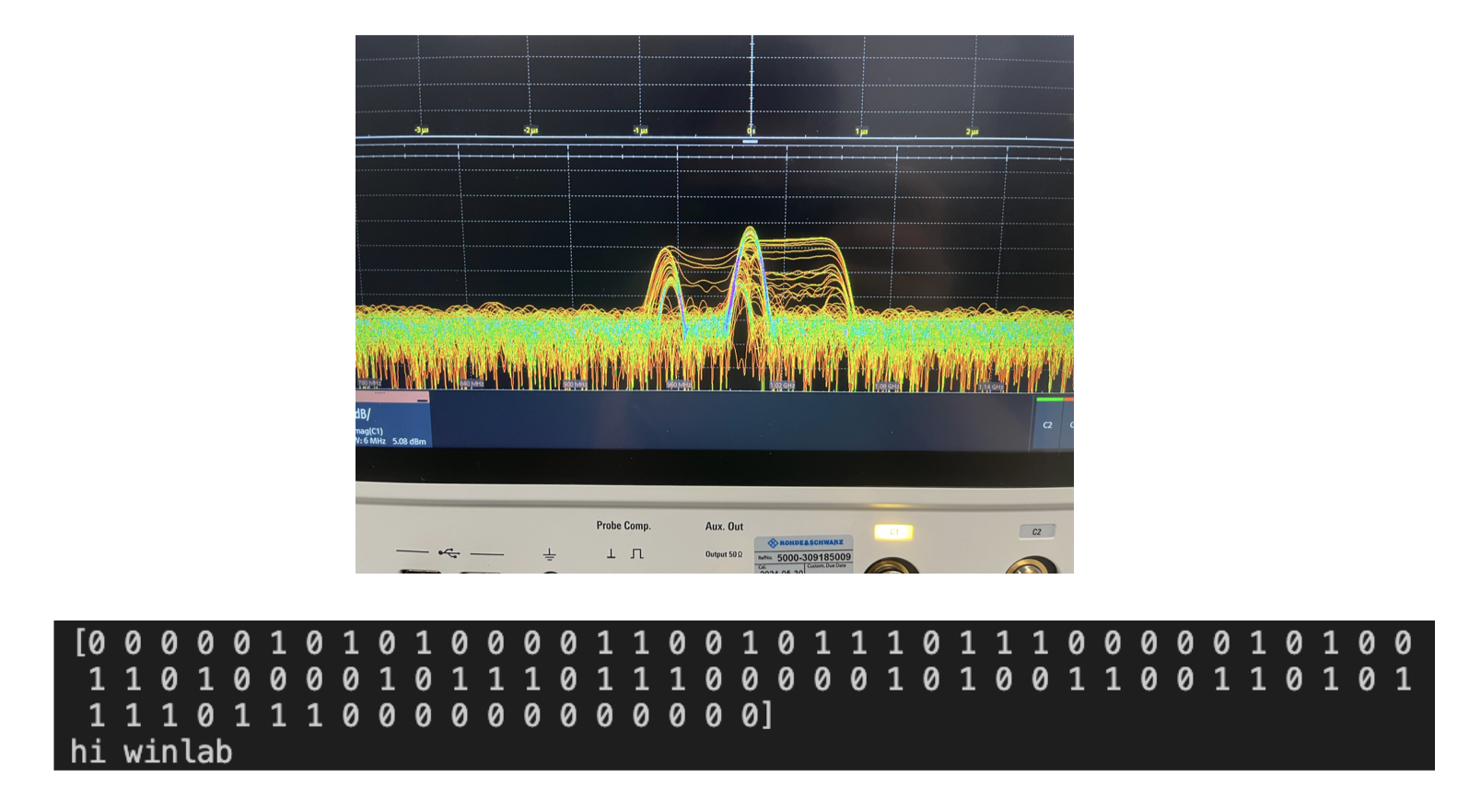
Earlier we saw BPSK working and get our message "hiii" back. We can do the same for OFDM. Here we receive our message "hi winlab"

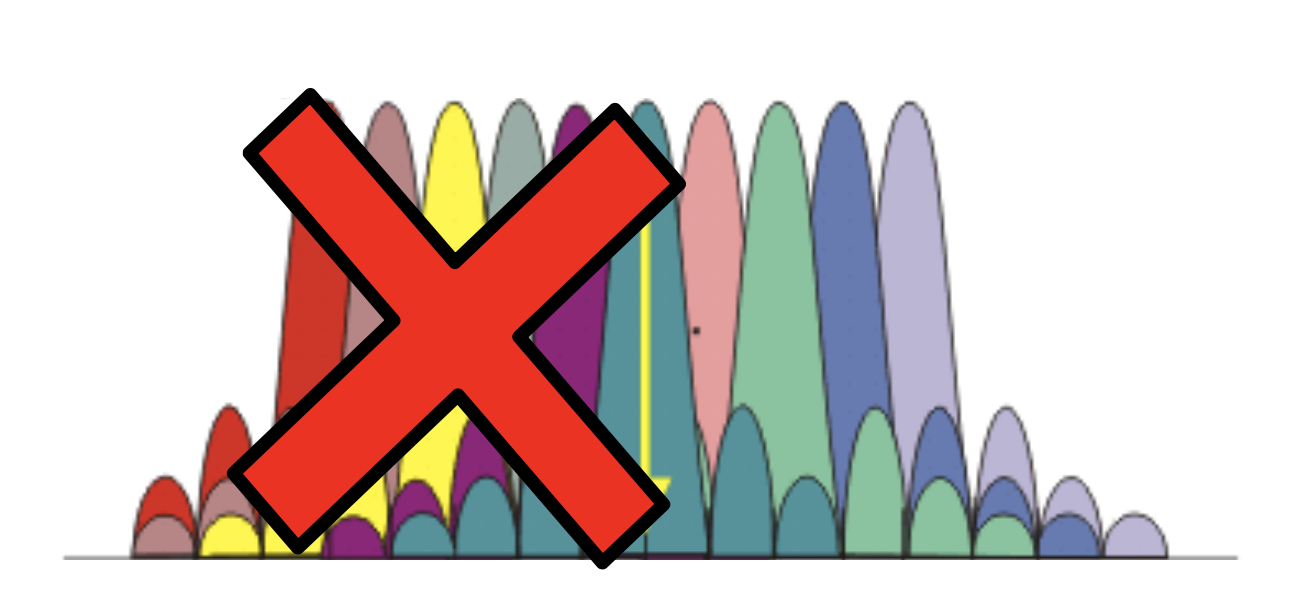
The ultimate goal is to send the two signals and see how they interact. This can very easily done by first blocking out the carriers we don't want to use in OFDM, then combining the signals simply by adding them.

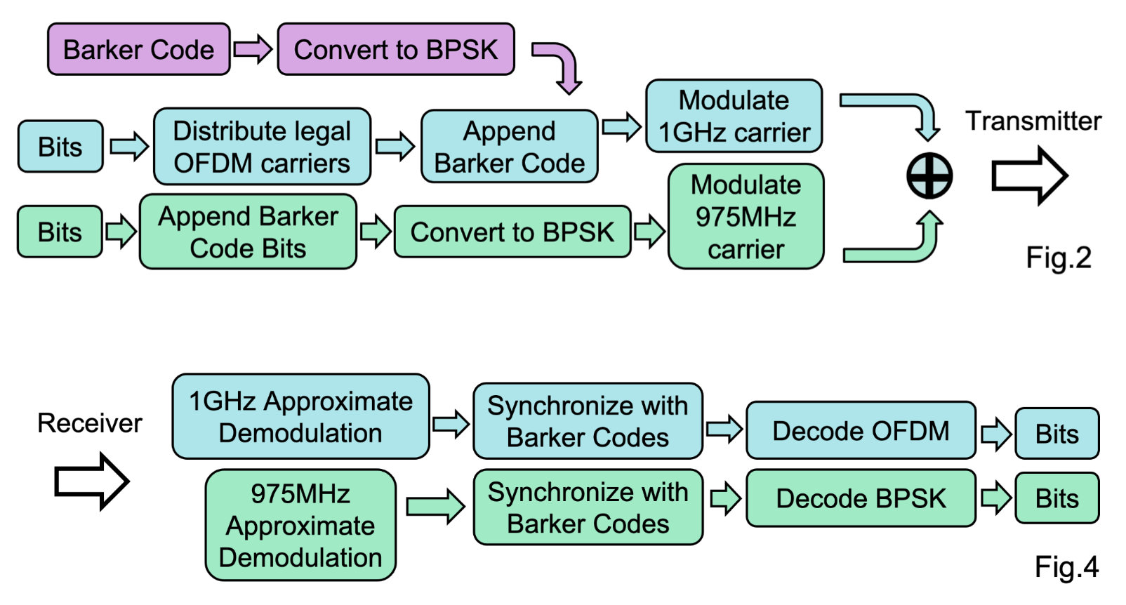
Below is also the architecture for the entire transmission and reception process.

Now when we try to read the signals. We can still read the BPSK, but get garbage from the OFDM.

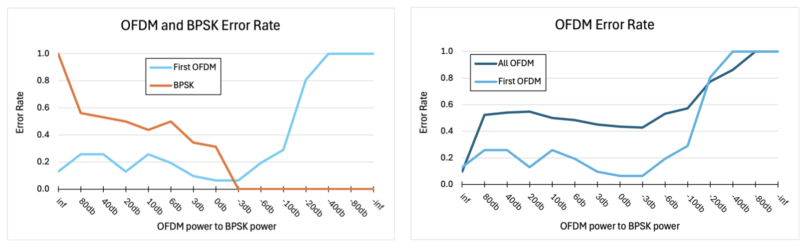
Here is also the error rates when OFDM and BPSK are at different levels.

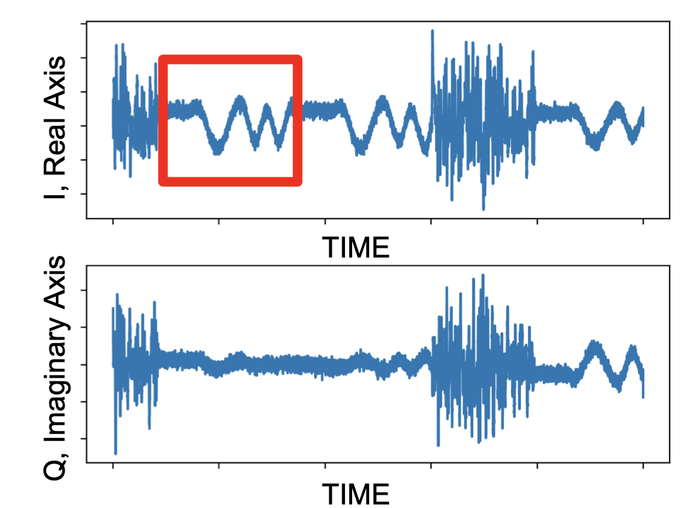
We sent OFDM in 4 consecutive groups. Because the synchronization is interfered with, the first group is read ok, but the subsequent ones fail.
Final Regards
Attachments (22)
- IMG_3524.JPG (3.3 MB ) - added by 2 years ago.
- Screen Shot 2024-08-06 at 10.32.22 AM.png (104.7 KB ) - added by 2 years ago.
- Screen Shot 2024-08-06 at 10.40.56 AM.png (266.3 KB ) - added by 2 years ago.
- Screen Shot 2024-08-06 at 3.01.41 PM.png (158.0 KB ) - added by 2 years ago.
- Screen Shot 2024-08-06 at 3.01.51 PM.png (191.0 KB ) - added by 2 years ago.
- Screen Shot 2024-08-06 at 2.31.04 PM.png (163.0 KB ) - added by 2 years ago.
- Screen Shot 2024-08-06 at 2.31.18 PM.png (187.7 KB ) - added by 2 years ago.
- Screen Shot 2024-08-06 at 3.02.06 PM.png (144.9 KB ) - added by 2 years ago.
- Screen Shot 2024-08-06 at 3.13.48 PM.png (244.6 KB ) - added by 2 years ago.
- Screen Shot 2024-08-06 at 3.14.10 PM.png (87.7 KB ) - added by 2 years ago.
- Screen Shot 2024-08-06 at 3.14.18 PM.png (275.9 KB ) - added by 2 years ago.
- Screen Shot 2024-08-06 at 3.18.35 PM.png (1.2 MB ) - added by 2 years ago.
- Screen Shot 2024-08-06 at 3.20.03 PM.png (322.4 KB ) - added by 2 years ago.
- Screen Shot 2024-08-06 at 5.44.33 PM.png (266.9 KB ) - added by 2 years ago.
- Screen Shot 2024-08-06 at 5.55.59 PM.png (174.1 KB ) - added by 2 years ago.
- Screen Shot 2024-08-06 at 6.03.54 PM.png (116.4 KB ) - added by 2 years ago.
- Screen Shot 2024-08-06 at 6.04.02 PM.png (60.2 KB ) - added by 2 years ago.
- Screen Shot 2024-08-06 at 6.38.04 PM.png (940.3 KB ) - added by 2 years ago.
- Screen Shot 2024-08-06 at 6.38.11 PM.png (271.8 KB ) - added by 2 years ago.
- Screen Shot 2024-08-06 at 6.38.20 PM.png (373.9 KB ) - added by 2 years ago.
- Screen Shot 2024-08-06 at 6.38.29 PM.png (1.1 MB ) - added by 2 years ago.
- Screen Shot 2024-08-06 at 6.38.38 PM.png (171.0 KB ) - added by 2 years ago.