Orbit > Tutorial > Analyzing Measurement Results

Analyzing Results

It is important to understand how measurements were collected and organized to be able to interpret them. The ORBIT Measurement Framework provides tools to insert points to tap available information and to effectively collect that information in a timely manner. And after the experiment is done, the user would get access to the exprimenet database generated. In general, the results of the experiment is in one ​MySQL database. Different participating nodes populate different tables of this database. Usually, user would like to post-process or visualize those raw measurements for further analysis.

A number of different tools are available to interpret experimental results. The choice of tools depends upon availability and the nature of the measurements. Excel and Matlab connections from your local laptop to our database server is blocked by the firewall. We are working on a system to safely and securely export databases to experimenters. Until then, please use any of the following approaches to retreive your data.

Note: Currently all databases share the same credentials.

Username and Password: orbit

Using MySQL Client

The easiest way to access your data is by manipulating the database directly with the MySQL Client. From gateway.orbit-lab.org (or any of the consoles), you may access your database by issuing the following commands from the command line:

$ mysql -h idb1 -u orbit -p
Enter password:
Welcome to the MySQL monitor.  Commands end with ; or \g.
Your MySQL connection id is 153 to server version: 4.1.15-Debian_1-log

Type 'help;' or '\h' for help. Type '\c' to clear the buffer.

mysql> use   <DB NAME>;

Standard MySQL queries can then be made to manipulate your data. A brief tutorial on how to use MySQL can be found ​here.

The database name is your experiment ID and is displayed by the nodehandler in the first few lines of your experiment run. It will look something like this:

 INFO init: Experiment ID: sb5_2006_01_17_11_45_23

Using Perl scripts

Sample Perl script that gets data from the database:

#! /usr/bin/perl
#
# Script: getdata.pl
# A simple script that gets all the rows from a single table in the database.
#
# ./getdata.pl <db_name> <table_name> <outputfile>
#
# Example: ./getdata.pl zmac1_2005_04_28_00_46_10  sender_otg_senderport  out.txt
#
# To use this script replace the XXXX in DBUSER and DBPASS
# with correct username and password for idb1.
#
#
use DBI();

$DBHOST = "idb1";
$DBNAME = $ARGV[0];
$DBUSER = "XXXX";
$DBPASS = "XXXX";
$QUERY = "select * from $ARGV[1]";
$OUTFILE = $ARGV[2];

$dsn = "DBI:mysql:database=$DBNAME;host=$DBHOST";

#Connect to the DB
$dbh = DBI->connect($dsn, $DBUSER, $DBPASS, {'RaiseError' => 1});

# Prepare and execute query
my $qry = $dbh->prepare($QUERY);
$qry->execute();

open(out, ">$OUTFILE");

#Print the column names
print out "@{$qry->{'NAME'}} \n";

#Print the data
while (my @ref = $qry->fetchrow()) {
        print out "@ref \n";
}

$qry->finish();
# Disconnect from the database.
$dbh->disconnect();

A more specific Perl script for OTG/OTR application can be found here

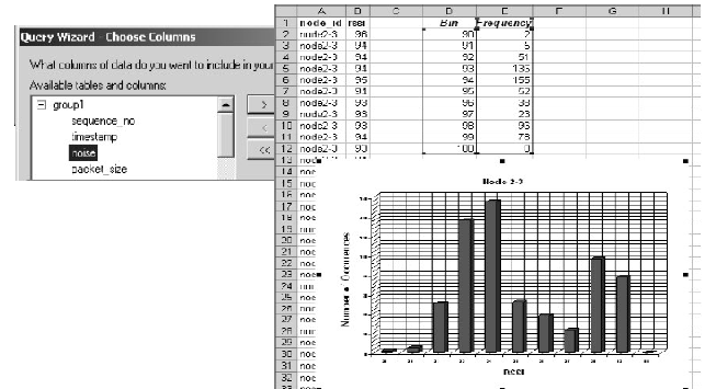
Using Microsoft Excel

Microsoft Excel can be used to analyze an experiment as shown below.

The user could import MySQL database to Microsoft Excel and use chart and other tools to analyze the measurements.

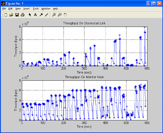
Using Matlab

Matlab is another tool can be used. It should be noted that the this assumes you have ​exported the database off of ORBIT and imported to your own MySQL server.

function nsf(dbServer, dbUser, dbPW, database);
% Part where we retrieve data from the database;
mysql('open',dbServer, dbUser, dbPW);
mysql('use', database);
output = struct('time',[],'thr_all',[],'node',[]);
[output.time, output.thr_all, output.node] = mysql('select timestamp, throughput, node_id from group2');
[thru1_4, time1_4, thru3_1, time3_1] = sort_mysql(output);
% Finally, the plotting part
subplot(2,1,1);
plot(time1_4, thru1_4, '-*');
title('Throughput On Obstructed Link');
xlabel('Time (sec)'); ylabel('Throuhput (bps)'); grid on;
subplot(2,1,2);
plot(time3_1, thru3_1, '-*');
title('Throughput On Monitor Node'); xlabel('Time (sec)');
ylabel('Throuhput (bps)'); grid on;

And the resulting graph is show below: