
| Version 138 (modified by , 9 years ago) ( diff ) |
|---|
Indoor Localization
Table of Contents
- 2015 Winlab Summer Internship
- LTE Unlicensed (LTE-U)
- Introduction
- Objectives
- Theory
- Analyzing Tools
- Experiment 1: Transmit and Receive LTE Signal
- Experiment 2: The Waterfall Plot
- Experiment 3: eNB and UE GUI
- Experiment 4: Varying Bandwidths
- Experiment 5: Working with TDD or FDD
- Experiment 6: TDD with Varying Bandwidths
- Experiment 7: TDD Waterfall Plot
- Poster
- Members
- Materials
- Resources
- LTE Unlicensed (LTE-U)
- Body Sensor Networks
- Dynamic Video Encoding
Introduction
The use of GPS services is growing just as fast as the development and accessibility of mobile devices. A GPS device, which used to be a significant investment, is now included in every smartphone that emerges on the market. These services have assisted many as they navigate themselves from place to place outdoors.
Although GPS is well-defined outdoors, localization indoors is still an active research problem. GPS signals indoors tend to be weaker; even if they are usable, the accuracy associated with GPS signals is not up to par. Large errors (on the order of meters) associated with GPS generally do not affect the user's ability to navigate to buildings, parks, landmarks, etc. Errors on the order of meters indoors, however, could mean that somebody is in a different room or different building altogether. A fine-grained service, down to the centimeter, is needed to localize indoors.
Motivation
An effective, low-cost, easy-to-implement solution to the indoor localization problem will have immediate impacts on everyday life, especially commercial retail. Based on movements of people in a store, retailers could determine where to place their best-selling items. They could place products effectively to accommodate shoppers and increase profits. In addition to commercial applications, indoor localization could help emergency responders efficiently respond to calls indoors, or help the elderly navigate inside a large building. Once the technology is fully developed, there are plenty of applications.
What is ORBIT Lab?
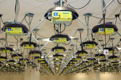
The ORBIT facility consists of a 20 x 20 grid of programmable radio nodes used to test wireless protocols and applications. Certain nodes in the facility, as well as certain sandboxes (part of the lab but not the grid), contain Universal Software Radio Peripherals (USRP), which are software defined radios that transmit and receive signals.

|
|
Founded in 2003 and launched in 2005, this lab provides the world's largest academic testbed for wireless communications. As of 2014, there are over 1000 registered users who have logged ~200,000 experimentation hours since the lab's founding.
Overall Approach

|
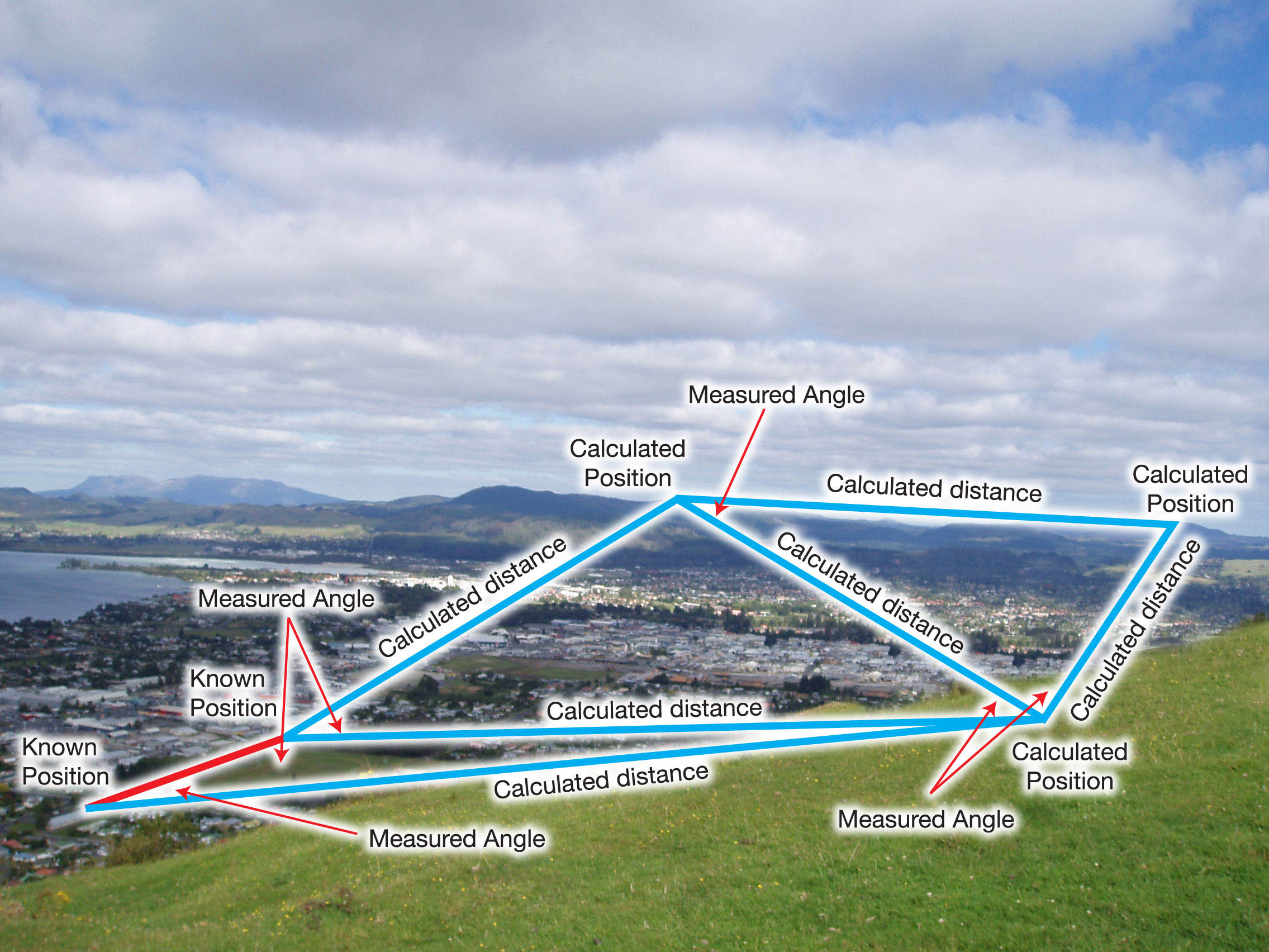
Trilateration is the method of determining location of an object through relative distances of points and geometry of spheres. It is a method that is used in Global Positioning Systems but we intend to use the same principle in indoor localization.
As illustrated below, knowing an object's relative distance from Boise, Minneapolis and Tucson, one can derive that that object is in Denver. Similarly, knowing a person's location from three USRPs enables us to roughly estimate his position in an indoor place.
||
|
|

|
|
|
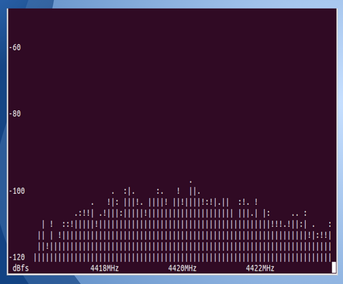
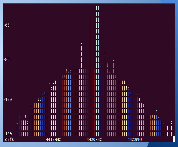
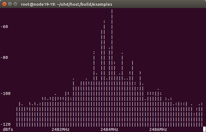
The photos below show what occurs before the signal is transmitted and after the signal is transmitted. The ASCII art below gives us a general idea of the signal amplitude, which is then measure directly with OMF (ORBIT Management Framework) commands.

|

|
|
|
|
|
|
| Analysis: The left image shows signal reception when there is no signal transmitted. This is the noise that is present while we conduct experiments in the ORBIT room. The peak that is visible in the right image is the frequency that the transmitted signal is received at the receiver nodes. |
|
|
|
|
|
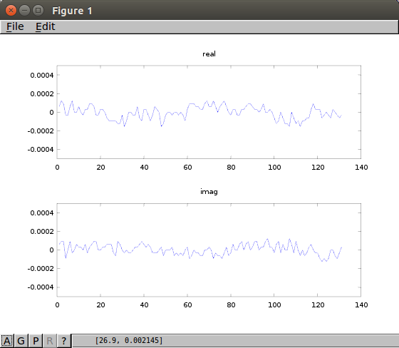
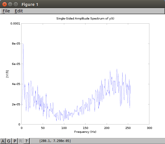
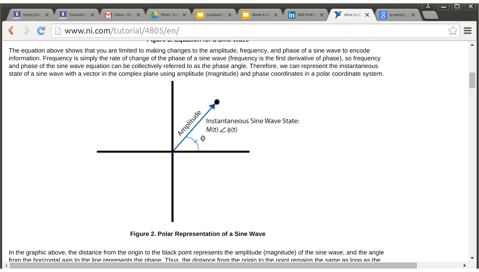
Analysis: We used USRPs to collect the IQ samples that are portrayed in Figure 1. The graph has time on the x axis and amplitude on the y axis for both the real and imaginary components of the signal. Figure 2 verifies the reception of this signal using Fast Fourier Transform in Matlab. IQ samples are often used for modulation and demodulation of the signal that is being analyzed. We used these samples to calculate the power of the signal at known distances.
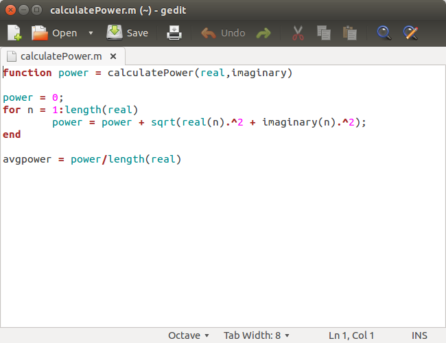
Experiment Three: Calculating powerCalculating signal amplitude and power is the next step in the process. The IQ samples, as mentioned above, gives the real and imaginary amplitude (y-axis) as it is related to time. Therefore, using the real amplitude on the x axis and the imaginary amplitude on the y-axis would result in the amplitude of the signal at a given time (hypotenuse). We can also calculate power from the similar calculation.

|

|
|
|
|
Experiment four: Relating SNR and power to distance
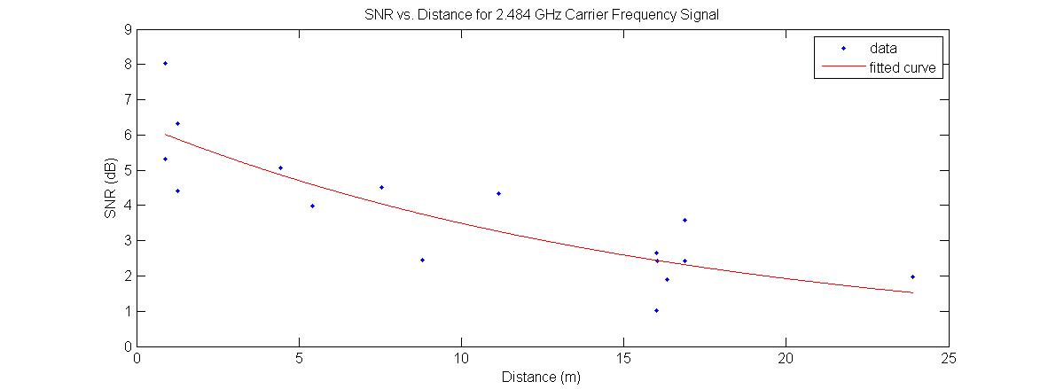
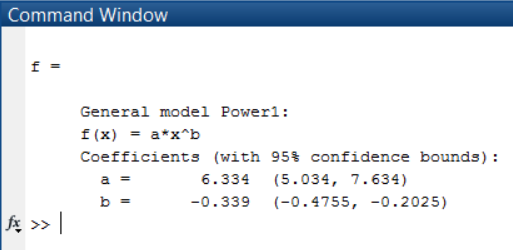
Signal to noise ratio is an important part in this localization process. To maintain a high SNR at higher distances means a greater chance of better localization data since there is more signal to collect and analyze. Even in the real world, people look for gadgets and devices with a higher SNR since that provides them with greater aural experience. Due to these reasons, it is very important to analyze SNR to validate the results and conclusions of the experiments.
|

|
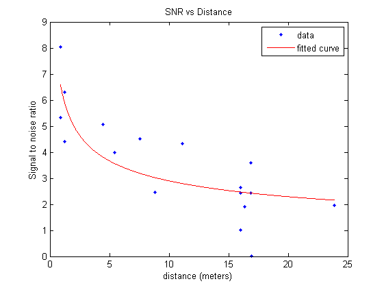
| Signal-to-Noise ratio versus distance and the fitted curve(red) |
|
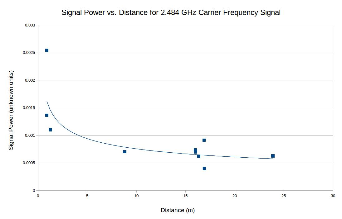
Analysis: Using the measured signal power, along with the distance between the transmitted and receiver, we obtained a signal amplitude-distance pair. We many of these pairs using different transmitters and receivers. We then plotted these items on a graph and found the exponential fit for the graph. As shown in this experiment, the line of best fit follows a generally negative and exponential curve but some of the points are no where close to the curve. However, the scattering of the data points signify either an error in signal processing or simply not enough data points in these graphs. We believed the latter might have had a hand in this error.
Experiment five: More IQ samples and updating SNR vs distance graph
As mentioned above, signal to noise ratio is very important since it relates signal quality as distance between receiver and transmitter increases. Therefore, it is important to gain points at smaller distance increments to certify that accurate data and best fit results are obtained. We obtained signal power and noise amplitude at certain distances that were not accounted before and graphed the data again.

|
|
|
|
|
|
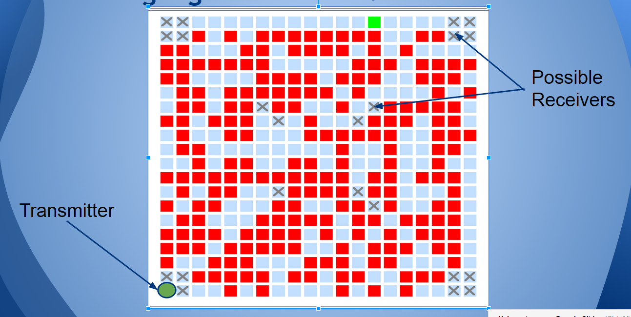
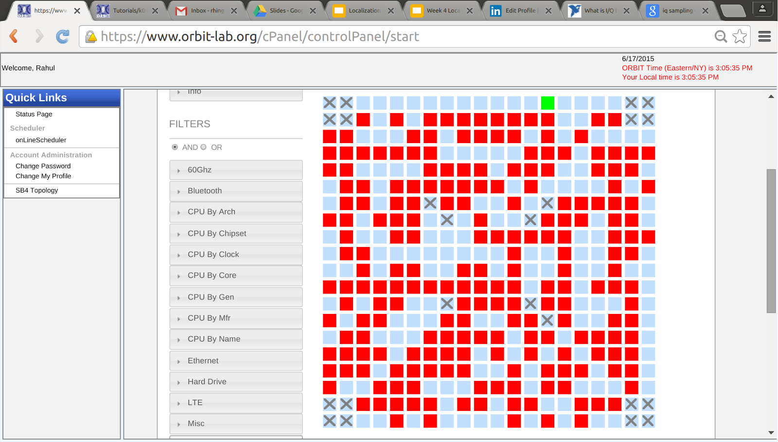
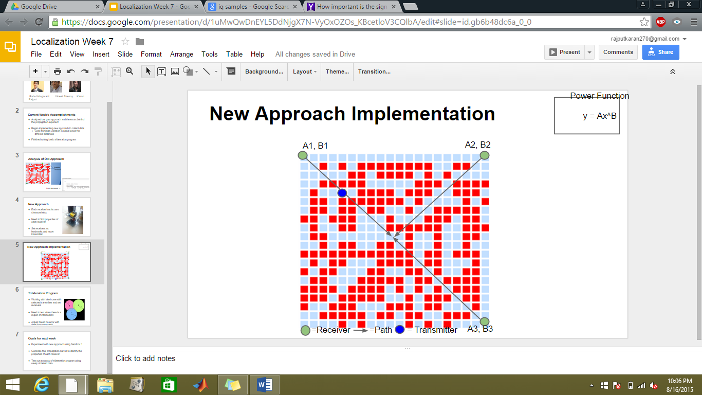
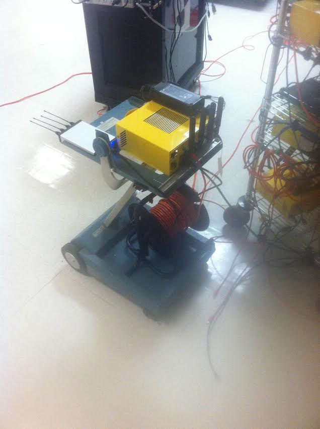
Analysis: The left picture shows the board that we are using to gain our signal power and noise amplitudes during this experiment. We used one transmitter as a control and several receivers. All the "X"s in the grid are transceivers, meaning that they can be used as either a transmitter or receiver. The picture on the right is a result of the experiment. We filled in certain holes by placing the receiver and the transmitter at certain known decisions and sending signals. As seen, the curve is a better fit of the data points but there are still points that are way off the chart and the graph is still scattered. We must have more controls to figure out the problem, so we decided to test all receivers. |
Experiment Six: Properties of each receiver
It is possible that using each of the USRP nodes interchangeably as a transmitter or a receiver was a source of error in the experiments. Each of the nodes may have had different properties to them so they might transmit or receive signals in a completely different way. Not to mention that they might get especially awry when they are used as a transmitter at one point and then as a receiver at another. Hence the properties of each of the receivers are studied.

|

|
|
|
|
Experiment Seven: Transmitter Calibration
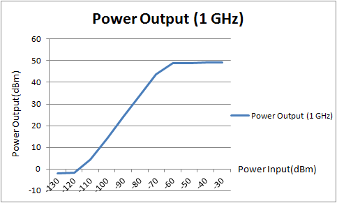
Calibration of the nodes is an important step if we are to get better localisation data and results. We have to make sure that the transmitters are transmitting the signals at the set frequency; any other frequency would offset the data. Therefore, we decided to see the difference in signal transmitting when connecting the node to a spectrum analyzer versus antenna to antenna transmission.
|
|
|
|
|
|
Experiment Eight: Receiver Calibration
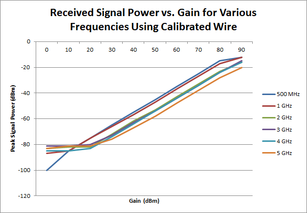
Calibrating the receivers is equally as important as calibrating the transmitters. The receiver was calibrated using a signal generator, a 30 dBm attenuator wire and wiserd. This calibration was to ensure that the power input and output was better hence giving us better signal power to distance data.

|

|
|
|
|
Plan of Action
1) Simultaneously obtain signal power values using Wiserd from all 3 receiver nodes2) Use calibration curves to convert Wiserd values to known dBm values
3) Use propagation curves to associate dBm value with a distance
4) Insert distances into trilateration program and obtain location of transmitter
Results and Conclusions
We used a trilateration program to analyze the data collected from these calibrated devices. The trilateration takes in 9 distance as inputs (3 distances from each receiver at 3 frequencies) and gives the location of the transmitter as the output. It does so but drawing three circles with the distance readings set as the radii and finds the intersection.
Our recent results have shown that if the transmitter is close to the center of the grid, the localization is most accurate. More data is necessary to come to any conclusions about accuracy of the program and results.
Transmitter Placed at (7.12, 6.4) m
Trilateration Estimate: (7.92, 8.19) m
Error: 1.75 m
Transmitter Placed at (2.25, 2.04) m
Trilateration Estimate: (5.77, 4.42) m
Error : 4.25 m
The project is no where closer to completion. Indoor localization is a topic that has been worked on for years now. For any effective method to be finalized, accurate results and collaboration are key. More work will be done on our project in the near future and updates will be posted on this page regularly.
Weekly Presentations
Presentations are done on a weekly basis before other research interns or professors. Presentations include the group's accomplishments over the past week as well as goals for the following week
Week 2
Week 3
Week 4
Week 5
Week 6
Week 7
Week 8
Week 9
Week 10
Week 11
Team

|

|

|
| Rahul Hingorani University of Michigan Industrial/Electrical Engineering |
Vineet Shenoy Rutgers University Electrical and Computer Engineering |
Karan Rajput Rutgers University Electrical and Computer Engineering |
Attachments (30)
- Rahul.png (16.1 KB ) - added by 9 years ago.
- Vineet.png (85.9 KB ) - added by 9 years ago.
- Karan.png (193.7 KB ) - added by 9 years ago.
- Localization Week 2.pdf (218.2 KB ) - added by 9 years ago.
- Localization Week 3.pdf (2.7 MB ) - added by 9 years ago.
- Week 4 Localization.pdf (1.8 MB ) - added by 9 years ago.
-
Orbit lab.jpg
(27.8 KB
) - added by 9 years ago.
Orbit lab photo
-
orbit_banner.png
(6.0 KB
) - added by 9 years ago.
Orbit banner
-
gridLocations.png
(326.8 KB
) - added by 9 years ago.
Grid Location of Transmitter and Receiver
-
Noise.png
(94.9 KB
) - added by 9 years ago.
Orbit Noise
-
Signal.png
(99.6 KB
) - added by 9 years ago.
Orbit Signal
- SNR vs Dist.png (4.6 KB ) - added by 9 years ago.
- SNR fit.png (23.2 KB ) - added by 9 years ago.
- triangulation.jpg (429.6 KB ) - added by 9 years ago.
- trilateration.gif (4.7 KB ) - added by 9 years ago.
- i-q1.png (26.5 KB ) - added by 9 years ago.
- i-q2.png (21.9 KB ) - added by 9 years ago.
- i-q3.png (29.3 KB ) - added by 9 years ago.
- amp.png (275.6 KB ) - added by 9 years ago.
- power.png (53.6 KB ) - added by 9 years ago.
- povdis.png (121.7 KB ) - added by 9 years ago.
- updatedgraph.png (72.4 KB ) - added by 9 years ago.
- newboard.png (248.3 KB ) - added by 9 years ago.
- latestapp.png (252.6 KB ) - added by 9 years ago.
- sandbox.png (936.9 KB ) - added by 9 years ago.
- trans.png (30.7 KB ) - added by 9 years ago.
- compare.png (29.2 KB ) - added by 9 years ago.
- oneghz.png (13.5 KB ) - added by 9 years ago.
- theovsreal.png (29.5 KB ) - added by 9 years ago.
- plan.png (454.8 KB ) - added by 9 years ago.
Download in other formats:
Powered by Trac 1.4.1
By Edgewall Software
.
Visit the Trac open source project at
https://trac.edgewall.org/